Introduction
This lecture will introduce how to scale up our algorithm to real practical RL problems by value function approximation.
Reinforcement learning can be used to solve large problems, e.g.
- Backgammon: \(10^{20}\) states
- Computer Go: \(10^{170}\) states
- Helicopter: continuous state space
How can we scale up the model-free methods for prediction and control from the last two lectures?
So far we have represented value function by a lookup table:
- Every state \(s\) has an entry \(V(s)\)
- Or every state-action pair \(s, a\) has an entry \(Q(s, a)\)
Problems with large MDPs:
- There are too many states and/or actions to store in memory
- It is too slow to learn the value of each state individually
Solution for large MDPs: Estimate value function with function approximation \[ \hat{v}(s, \mathbb{w})\approx v_\pi(s)\\ \mbox{or }\hat{q}(s, a, \mathbb{w})\approx q_\pi(s, a) \] where \(\hat{v}\) or \(\hat{q}\) are function approximations of real \(v_\pi\) or \(q_\pi\), and \(\mathbb{w}\) are the parameters. This apporach has a major advantage:
- Generalise from seen state to unseen states
We can fit the \(\hat{v}\) or \(\hat{q}\) to \(v_\pi\) or \(q_\pi\) by MC or TD learning.
Types of Value Function Approximation
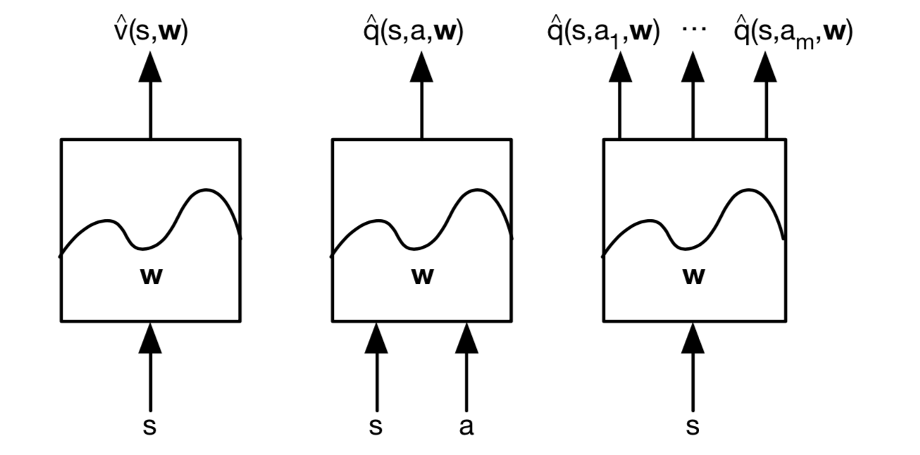
We consider \(\color{red}{\mbox{differentiable}}\) function approximators, e.g.
- Linear combinations of features
- Neural network
Futhermore, we require a training method that is suitable for \(\color{red}{\mbox{non-stationary}}\), \(\color{red}{\mbox{non-idd}}\) (idd = independent and identical distributed) data.
Table of Contents
Incremental Methods
Value Function Approximation
Gradient Descent
Let \(J(\mathbb{w})\) be a differentiable function of parameter vector \(\mathbb{w}\).
Define the gradient of \(J(\mathbb{w})\) to be \[ \bigtriangledown_wJ(\mathbb{w})=\begin{pmatrix} \frac{\partial J(\mathbb{w})}{\partial \mathbb{w}_1} \\ \vdots\\ \frac{\partial J(\mathbb{w})}{\partial \mathbb{w}_n} \end{pmatrix} \] To find a local minimum of \(J(\mathbb{w})\), adjust \(\mathbb{w}\) in direction of -ve gradient \[ \triangle \mathbb{w}=-\frac{1}{2}\alpha \bigtriangledown_\mathbb{w}J(\mathbb{w}) \] where \(\alpha\) is a step-size parameter.
So let's apply the stochastic gradient descent to value fucntion approximation.
Goal: find parameter vector \(\mathbb{w}\) minimising mean-squared error between approximate value function \(\hat{v}(s, \mathbb{w})\) and true value function \(v_\pi(s)\). \[ J(\mathbb{w})=\mathbb{E}_\pi[(v_\pi(S)-\hat{v}(S, \mathbb{w}))^2] \] Gradient descent finds a local minimum \[ \begin{align} \triangle\mathbb{w}&=-\frac{1}{2}\alpha \bigtriangledown_\mathbb{w}J(\mathbb{w})\\ & = \alpha\mathbb{E}_\pi[(v_\pi(S)-\hat{v}(S, \mathbb{w}))\bigtriangledown_\mathbb{w}\hat{v}(S, \mathbb{w})] \\ \end{align} \] Stochastic gradient descent samples the gradient \[ \triangle\mathbb{w}=\alpha(v_\pi(S)-\hat{v}(S, \mathbb{w}))\bigtriangledown_\mathbb{w}\hat{v}(S, \mathbb{w}) \] Expected update is equal to full gradient update.
Feature Vectors
Let's make this idea more concrete.
Represent state by a feature vector: \[ x(S) =\begin{pmatrix} x_1(S) \\ \vdots\\ x_n(S) \end{pmatrix} \] For example:
- Distance of robot from landmarks
- Trend in the stock market
- Piece and pawn configurations in chess
Linear Value Function Approximation
Represent value function by a linear combination of features \[ \hat{v}(S, \mathbb{w})=x(S)^T\mathbb{w}=\sum^n_{j=1}x_j(S)\mathbb{w}_j \] Objective function is quadratic in parameters \(\mathbb{w}\) \[ J(\mathbb{w})=\mathbb{E}_\pi[(v_\pi(S)-x(S)^T\mathbb{w})^2] \] Stochastic gradient descent converges on global optimum.
Update rule is particularly simple \[ \bigtriangledown_\mathbb{w}\hat{v}(S, \mathbb{w})=x(S)\\ \triangle \mathbb{w}=\alpha(v_\pi(S)-\hat{v}(S, \mathbb{w}))x(S) \] Update = step-size \(\times\) prediction error \(\times\) feature value.
So far we have assumed true value function \(v_\pi(s)\) given by supervisor. But in RL there is no supervisor, only rewards.
In practice, we substitute a target for \(v_\pi(s)\):
For MC, the target is return \(G_t\) \[ \triangle \mathbb{w}=\alpha(\color{red}{G_t}-\hat{v}(S_t, \mathbb{w}))\bigtriangledown_w \hat{v}(S_t, \mathbb{w}) \]
For TD(0), the target is the TD target \(R_{t+1}+\gamma\hat{v}(S_{t+1}, \mathbb{w})\) \[ \triangle \mathbb{w}=\alpha(\color{red}{R_{t+1}+\gamma\hat{v}(S_{t+1}, \mathbb{w})}-\hat{v}(S_t, \mathbb{w}))\bigtriangledown_w \hat{v}(S_t, \mathbb{w}) \]
For TD(\(\lambda\)), the target is the return \(G_t^\lambda\) \[ \triangle \mathbb{w}=\alpha(\color{red}{G_t^\lambda}-\hat{v}(S_t, \mathbb{w}))\bigtriangledown_w \hat{v}(S_t, \mathbb{w}) \]
Monte-Carlo with Value Function Approximation
Return \(G_t\) is unbiased, noisy sample of true value \(v_\pi(S_t)\). We can build our "training data" to apply supervised learning: \[ <S_1, G_1>, <S_2, G_2>, ..., <S_T, G_T> \] For example, using linear Monte-Carlo policy evaluation \[ \begin{align} \triangle \mathbb{w}&=\alpha(\color{red}{G_t}-\hat{v}(S_t, \mathbb{w}))\bigtriangledown_w \hat{v}(S_t, \mathbb{w}) \\ & = \alpha(G_t-\hat{v}(S_t, \mathbb{w}))x(S_t)\\ \end{align} \] Monte-Carlo evaluation converges to a local optimum even when using non-linear value function approximation.
TD Learning with Value Function Approximation
The TD-target \(R_{t+1}+\gamma \hat{v}(S_{t+1}, \mathbb{w})\) is a biased sample of true value \(v_\pi(S_t)\). We can still apply supervised learning to "traning data": \[ <S_1, R_2 +\gamma\hat{v}(S_2, \mathbb{w})>,<S_2, R_3 +\gamma\hat{v}(S_3, \mathbb{w})>,...,<S_{T-1}, R_T> \] For example, using linear TD(0) \[ \begin{align} \triangle \mathbb{w}&=\alpha(\color{red}{R+\gamma\hat{v}(S', \mathbb{w})}-\hat{v}(S, \mathbb{w}))\bigtriangledown_w \hat{v}(S, \mathbb{w}) \\ & = \alpha\delta x(S)\\ \end{align} \] Linear TD(0) converges (close) to global optimum.
TD(\(\lambda\)) with Value Function Approximation
The \(\lambda\)-return \(G_t^\lambda\) is also a biased sample of true value \(v_\pi(s)\). We can also apply supervised learning to "training data": \[ <S_1, G_1^\lambda>, <S_2, G_2^\lambda>, ..., <S_{T-1}, G_{T-1}^\lambda> \] Can use either forward view linear TD(\(\lambda\)): \[ \begin{align} \triangle \mathbb{w}&=\alpha(\color{red}{G_t^\lambda}-\hat{v}(S_t, \mathbb{w}))\bigtriangledown_w \hat{v}(S_t, \mathbb{w}) \\ & = \alpha(G_t-\hat{v}(S_t, \mathbb{w}))x(S_t)\\ \end{align} \] or backward view linear TD(\(\lambda\)): \[ \begin{align} \delta_t &= R_{t+1}+\gamma \hat{v}(S_{t+1}, \mathbb{w})-\hat{v}(S_t, \mathbb{w}) \\ E_t& = \gamma\lambda E_{t-1} +x(S_t) \\ \triangle\mathbb{w}&=\alpha\delta_tE_t \end{align} \]
Action-Value Function Approximation
Approximate the action-value function: \[ \hat{q}(S, A, \mathbb{w}) \approx q_\pi(S, A) \] Minimise mean-squared error between approximate action-value function \(\hat{q}(S, A, \mathbb{w})\) and true action-value function \(q_\pi(S, A)\): \[ J(\mathbb{w})=\mathbb{E}_\pi[(q_\pi(S, A)-\hat{q}(S, A, \mathbb{w}))^2] \] Use stochastic gradient descent to find a local minimum: \[ -\frac{1}{2}\bigtriangledown_w J(\mathbb{w})=(q_\pi(S, A)-\hat{q}(S, A, \mathbb{w}))\bigtriangledown_w\hat{q}(S, A, \mathbb{w})\\ \triangle\mathbb{w}=\alpha (q_\pi(S, A)-\hat{q}(S, A, \mathbb{w}))\bigtriangledown_w\hat{q}(S, A, \mathbb{w}) \] Represent state and action by a feature vector: \[ \mathbb{x}(S, A)=\begin{pmatrix} x_1(S, A) \\ \vdots\\ x_n(S, A) \end{pmatrix} \] Represent action-value function by linear combination of features: \[ \hat{q}(S, A, \mathbb{w})=\mathbb{x}(S, A)^T\mathbb{w}=\sum^n_{j=1}x_j (S, A)\mathbb{w}_j \] Stochastic gradient descent update: \[ \bigtriangledown_w\hat{q}(S, A, \mathbb{w})=\mathbb{x}(S, A)\\ \triangle \mathbb{w}=\alpha(q_\pi(S, A)-\hat{q}(S, A, \mathbb{w}))\mathbb{x}(S, A) \] Like prediction, we must subsitute a target for \(q_\pi(S, A)\):
For MC, the target is the return \(G_t\) \[ \triangle \mathbb{w}=\alpha(\color{red}{G_t}-\hat{q}(S_t, A_t, \mathbb{w}))\bigtriangledown_w\hat{q}(S_t, A_t, \mathbb{w}) \]
For TD(0), the target is the TD target \(R_{t+1}+\gamma Q(S_{t+1}, A_{t+1})\) \[ \triangle \mathbb{w}=\alpha(\color{red}{R_{t+1}+\gamma \hat{q}(S_{t+1}, A_{t+1}, \mathbb{w})}-\hat{q}(S_t, A_t, \mathbb{w}))\bigtriangledown_w\hat{q}(S_t, A_t, \mathbb{w}) \]
For forward-view TD(\(\lambda\)), target is the action-value \(\lambda\)-return \[ \triangle\mathbb{w}=\alpha(\color{red}{q_t^\lambda}-\hat{q}(S_t, A_t,\mathbb{w}))\bigtriangledown\hat{q}(S_t, A_t, \mathbb{w}) \]
For backward-view TD(\(\lambda\)), equivalent update is \[ \begin{align} \delta_t& =R_{t+1}+\gamma\hat{q}(S_{t+1}, A_{t+1}, \mathbb{w})-\hat{q}(S_t, A_t, \mathbb{w}) \\ E_t& = \gamma\lambda E_{t-1}+\bigtriangledown_w\hat{q}(S_t, A_t, \mathbb{w}) \\ \triangle\mathbb{w}&= \alpha\delta_t E_t \end{align} \]
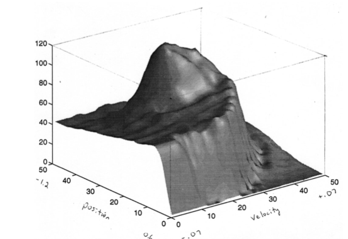
Linear Sarsa with Coarse Coding in Mountain Car
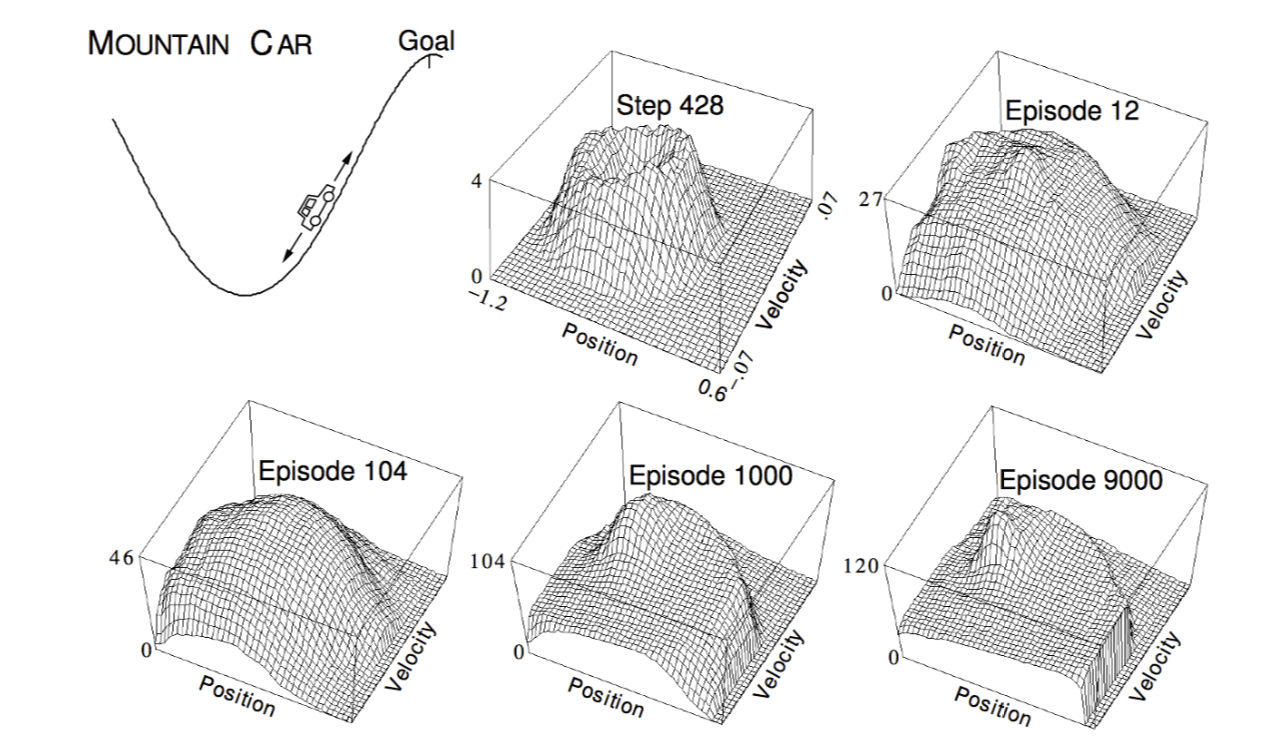
The goal is to control our car to reach the top of the mountain. We represent state by the car's position and velocity. The height of the diagram shows the value of each state. Finally, the value function is like:
Study of \(\lambda\): Should We Bootstrap?
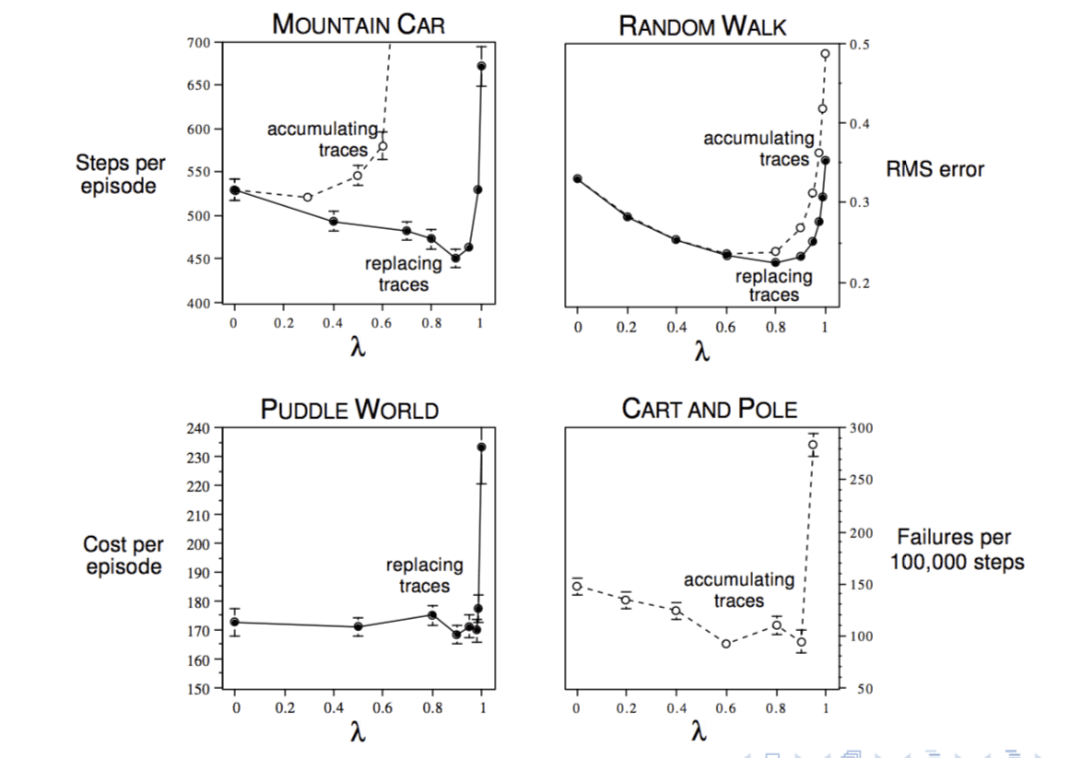
The answer is yes. We can see from above picture, choose some approprite \(\lambda\) can certainly reduce the training steps as well as the cost.
However, temporal-difference learning in many cases doesn't guarantee to converge. It may also diverge.
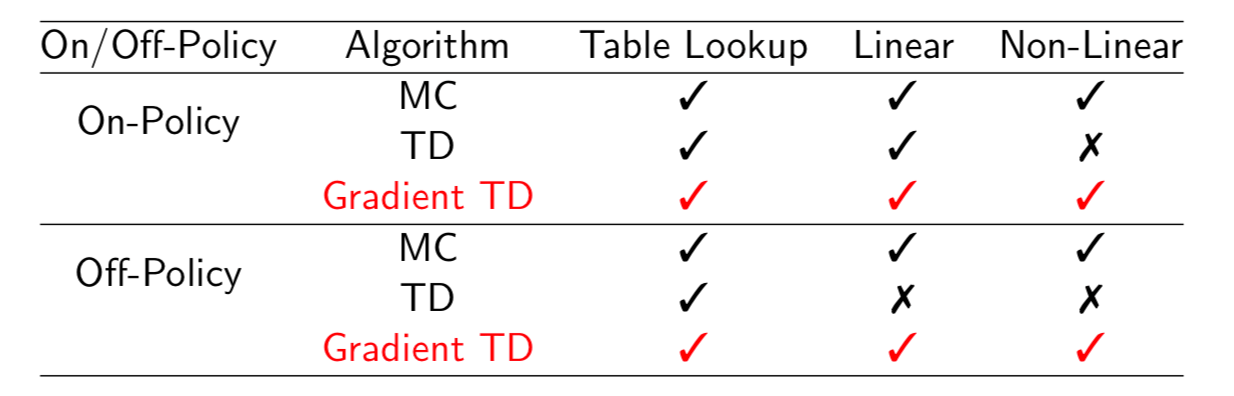
Convergence of Prediction Algorithms
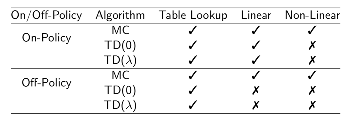
TD dose not follow the gradient of any objective function. This is why TD can diverge when off-policy or using non-linear function approximation. Gradient TD follows true gradient of projected Bellman error.
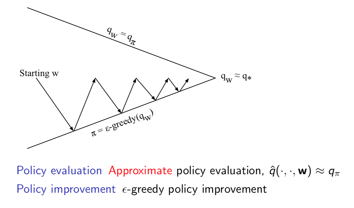
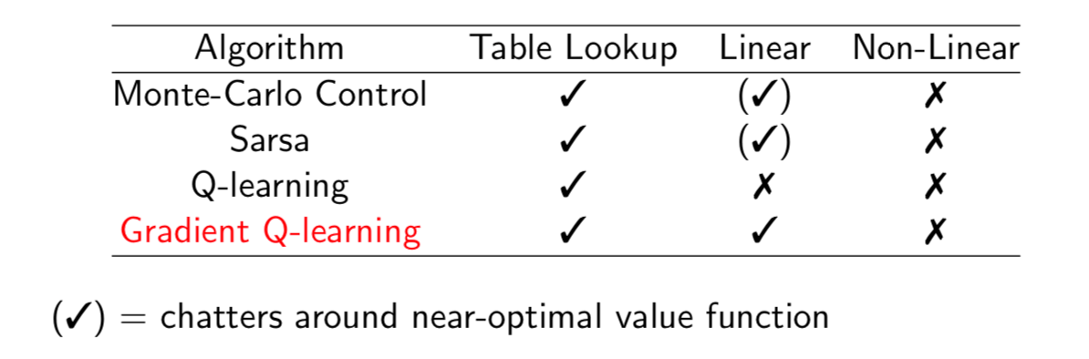
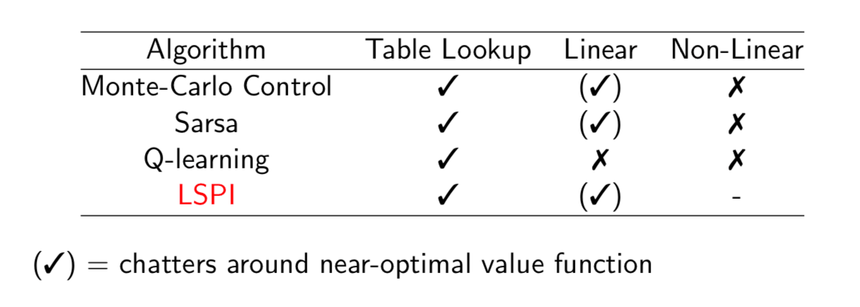
Convergence of Control Algorithms
Batch Methods
Gradient descent is simple and appealing. But it is not sample efficient. Batch methods seek to find the best fitting value function given the agent's experience.
Least Square Prediction
Give value function approximation \(\hat{v}(s, \mathbb{w})\approx v_\pi(s)\) and experience \(\mathcal{D}\) consisting of <state, value> pairs: \[ \mathcal{D} = \{<s_1, v_1^\pi>, <s_2, v_2^\pi>, ..., <s_T, v_T^\pi> \} \] Which parameters \(\mathbb{w}\) give the best fitting value function \(\hat{v}(s, \mathbb{w})\) ?
\(\color{red}{\mbox{Least squares}}\) algorithms find parameter vector \(\mathbb{w}\) minimising sum-squared error between \(\hat{v}(s_t, \mathbb{w})\) and target values \(v_t^\pi\), \[ \begin{align} LS(\mathbb{w}) & = \sum^T_{t=1}(v_t^\pi-\hat{v}(s_t, \mathbb{w}))^2 \\ & = \mathbb{E}_\mathcal{D}[(v^\pi-\hat{v}(s, \mathbb{w}))^2] \\ \end{align} \] Given experience consisting of <state, value> pairs \[ \mathcal{D}=\{<s_1, v_1^\pi>, <s_2, v_2^\pi>, ..., <s_T, v_T^\pi>\} \] Repeat:
Sample state, value from experience \[ <s, v^\pi> \sim \mathcal{D} \]
Apply stochastic gradient descent update \[ \triangle \mathbb{w}=\alpha(v^\pi-\hat{v}(s, \mathbb{w}))\bigtriangledown_w\hat{v}(s, w) \]
Converges to least squares solution \[ \mathbb{w}^\pi=\arg\min_w LS(w) \] Deep Q-Networks (DQN)
DQN uses \(\color{red}{\mbox{experience replay}}\) and \(\color{red}{\mbox{fixed Q-targets}}\):
Take action \(a_t\) according to \(\epsilon\)-greedy policy
Store transition \((s_t, a_t, r_{t+1}, s_{t+1})\) in replay memory \(\mathcal{D}\)
Sample random mini-batch of transitions \((s, a, r, s')\) from \(\mathcal{D}\)
Compute Q-learning targets w.r.t. old, fixed parameters \(w^-\)
Optimise MSE between Q-network and Q-learning target \[ \mathcal{L}(w_i)=\mathbb{E}_{s,a,r,s'\sim\mathcal{D}_i}[(r+\gamma\max_{a'}Q(s',a';w^-_i)-Q(s, a;w_i))^2] \]
Using variant of stochastic gradient descent
Note: \(\color{red}{\mbox{fixed Q-targets}}\) means we use two Q-networks. One of it using fixed old parameters to generate the Q-target to update the fresh Q-network, which can keep the update stable. Otherwise, when you update the Q-network, you also update the Q-target, which can cause diverge.
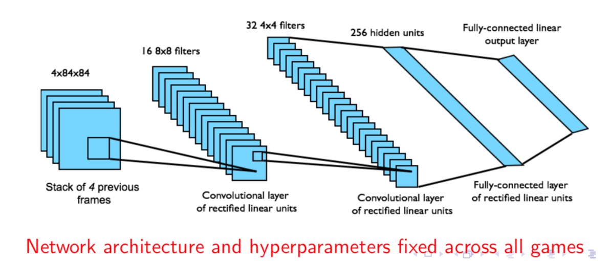
DQN in Atari
- End-to-end learning of values \(Q(s, a)\) from pixels \(s\)
- Input state \(s\) is stack of raw pixels from last 4 frames
- Output is \(Q(s, a)\) for 18 joystick/button positions
- Rewards is change in score for that step
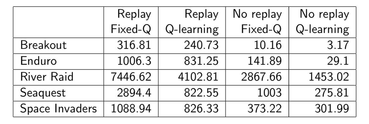
Results
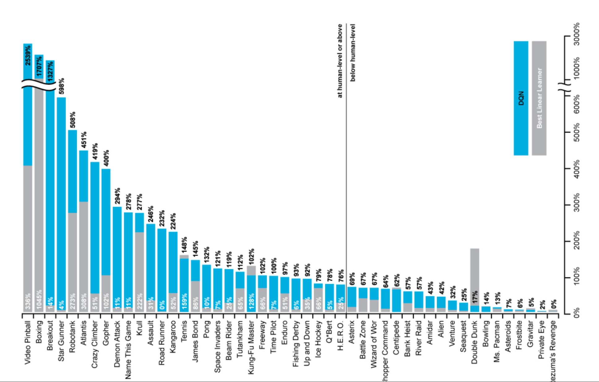
How much does DQN help?
Linear Least Squares Prediction - Normal Equation
Experience replay finds least squares solution but it may take many iterations. Using linear value function approximation \(\hat{v}(s, w) = x(s)^Tw\), we can solve squares soluton directly.
At minimum of \(LS(w)\), the expected update must be zero:
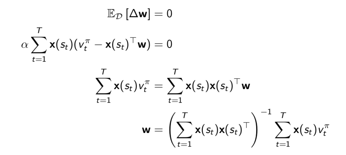
For \(N\) features, direct solution time is \(O(N^3)\). Incremental solution time is \(O(N^2)\) using Shermann-Morrison.
We do not know true values \(v_t^\pi\). In practice, our "training data" must be noisy or biased samples of \(v_t^\pi\):
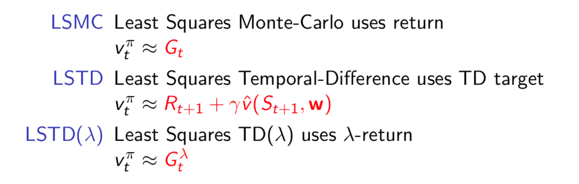
In each case solve directly for fixed point of MC / TD / TD(\(\lambda\)).
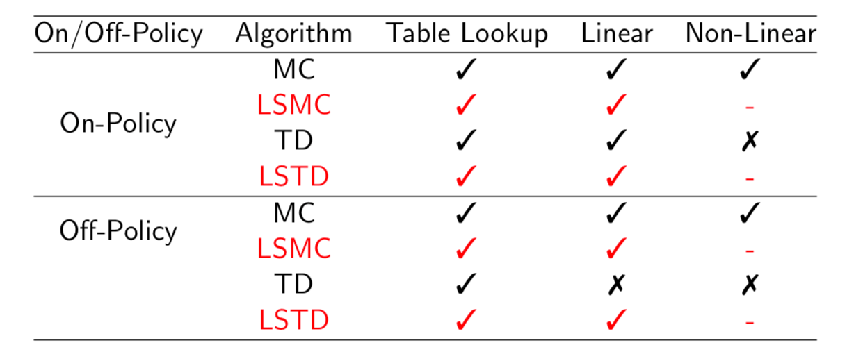
Convergence of Linear Least Squares Prediction Algorithms
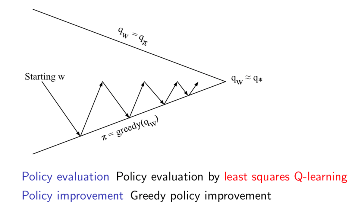
Least Squares Control
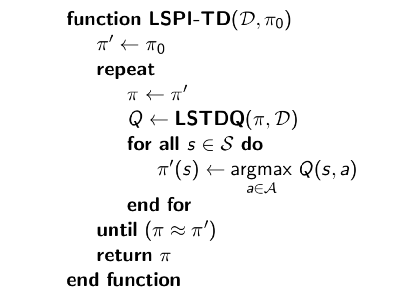
Least Squares Policy Iteration
Least Squares Action-Value Function Approximation
Approximate action-value function \(q_\pi(s, a)\) using linear combination of features \(\mathbb{x}(s, a)\): \[ \hat{q}(s, a, \mathbb{w})=\mathbb{x}(s, a)^T\mathbb{w}\approx q_\pi(s, a) \] Minimise least squares error between \(\hat{q}(s, a, \mathbb{w})\) and \(q_\pi(s, a)\) from experience generated using policy \(\pi\) consisting of <(state, action), value> pairs: \[ \mathcal{D}=\{<(s_1,a_1),v_1^\pi>,<(s_2,a_2),v_2^\pi>,...,<(s_T,a_T),v_T^\pi>\} \] Least Squares Control
For policy evaluation, we want to efficiently use all experience. For control, we also want to improve the policy. This experience is generated from many policies. So to evaluate \(q_\pi(S, A)\) we must learn \(\color{red}{\mbox{off-policy}}\).
We use the same idea as Q-learning:
- Use experience generated by old policy \(S_t, A_t, R_{t+1}, S_{t+1} \sim \pi_{old}\)
- Consider alternative successor action \(A'=\pi_{new}(S_{t+1})\)
- Update \(\hat{q}(S_t, A_t,\mathbb{w})\) towards value of alternative action \(R_{t+1}+\gamma \hat{q}(S_{t+1}, A', \mathbb{w})\)
Consider the following linear Q-learning update \[ \delta=R_{t+1}+\gamma \hat{q}(S_{t+1}, \color{red}{\pi(S_{t+1})}, \mathbb{w})-\hat{q}(S_t, A_t, \mathbb{w})\\ \triangle \mathbb{w}=\alpha\delta\mathbb{x}(S_t, A_t) \] LSTDQ algorithm: solve for total update = zero:
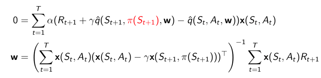
The following pseudocode uses LSTDQ for policy evaluation. It repeatedly re-evaluates experience \(\mathcal{D}\) with different policies.
Convergence of Control Algorithms
End.